Lee Altenberg's Home Page |
Curriculum Vitae |
Papers |
Evolved Graphics |
Sand Dune Ripples |
E-mail me
About this document ...
Evolutionary Computation Models
from Population Genetics:
Part 2: An Historical Toolbox
A Tutorial presented at the Congress on Evolutionary Computation, 2000
Lee Altenberg, Ph.D.
Information and Computer Sciences
University of Hawai`i at Manoa
http://dynamics.org/~altenber/
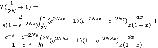
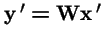
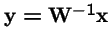
The Framework for Evolutionary Algorithms:
=
- Operators,
- (mutation, crossover, inversion, conversion, etc.) acting on the
- Representations
- of the search space (genotypes, strings, programs, designs, etc.), generate a
- Transmission function,
- the probability distribution of offspring types from any combination (one, two, etc., sometimes the whole population) of parent types.
- The relationship
- between the transmission function and the fitness function is the main determinant the performance of the evolutionary algorithm.
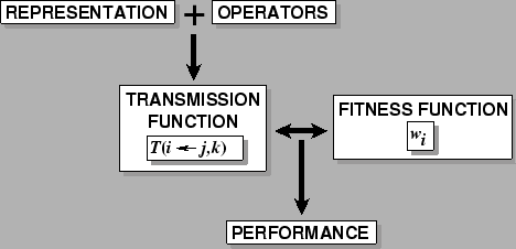
The Two Elements of Darwinian
Dynamics:
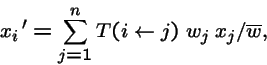
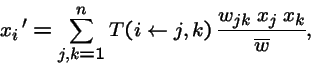
Where:
- i
- is an individual's type,
- xi
- is the frequency of type i in the population,
- wi
- is the fitness coefficient of type i, and
-

- is the probability that type j produces offspring of type i (i.e. transformation--mutation, recombination, migration, permutation, etc.).
-

- is when there are two parents, types j and k.
A population geneticist encounters
evolutionary computation:
``Fitness proportionate selection'' sounds like
``Velocity proportionate speed''
``Temperature proportionate heat''
``Mass proportionate weight''
``Length proportionate distance''
In other words, in evolutionary biology,
`Fitness' is the measure of selection.
Objective function (phenotype)  Fitness
A better term: `Proportional Fitness'
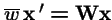
The selection operator can be expressed as:
or in vector form:
Q. Isn't
 only for `proportional selection'?
A. No: the coefficient wi needn't be constant:
In fact  can be functions of:
- the frequencies of types in the population,
- location,
- time,
- other species, agents, etc.--coevolution,
- or be a random variable.
Other biological components of Selection:
- Fitness Components:
-
- Viability (survival rate)
- Fecundity (offspring number)
- Fertility (offspring number of particular mating types)
- When multi-parameter fitness coefficients may be required:
-
- Survivorship curves -- age dependent survival
- Fecundity curves -- age dependent reproduction
- Gene
 Environment interactions
A Classification of Selection:
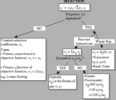
Q: Suppose there is an evolutionary game being played between the types in a population. Will the evolutionarily stable strategies (ESS) be the same whether you use constant (`proportional') selection, or truncation selection?
A: No! Illustrates the hazard of calling
uij the `fitnesses'.
Models of Canonical Evolutionary Algorithms:
- Lewontin, R. C. 1964. The interaction of selection and linkage: I. General considerations; heterotic models. Genetics 49: 49-67 (esp. pp. 55-56).
- Slatkin, M. 1970. Selection and polygenic characters. Proceedings of the National Academy of Sciences U.S.A. 66:
87-93.
Asexual:
or in vector form:
where
- xi = frequency of genotype xi in the population, and
 frequency in the next generation;
- wi = fitness of genotype i ;
-
 = probability that genetic operators produce offspring i from parent j; and
-
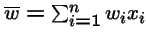 = mean fitness of the population.
Sexual
or in vector form:
(a quadratic operator--
 not tractable in general), where

- is the tensor product (see below);
- wij
- is the fitness of the parental pair (i,j)

- is the n2 by n2 diagonal matrix of coefficients
wi1 i2;
-
- = probability that genetic operators produce offspring i from parents j and k,
 ;
;

- in this case is the n by n2 matrix of transmission probabilities;
For haploid selection,
wi1 i2 = wi1 wi2 or
 , hence:
Solution for generic mutation and constant selection:
Q. What is the limit as
 ?
?
A. For generic mutation and selection:
One attractor, not multiple peaks.
Result 1
Suppose a mutation operator is ergodic: i.e. repeated application of the operator can mutate any genotype into any other genotype. Then, under an algorithm of constant selection and mutation, there is only one domain of attraction of the system--i.e. one `fitness peak'.
Perron-Frobenius Theory
How is this result derived?
Theorem 1 (Perron 1907, Frobenius)
If a matrix

,
or some power

,
has all positive entries, then:
- 1.
- The eigenvalue of
with the largest magnitude,
 (the `spectral radius'), is always real and positive, and strictly larger in magnitude that all other eigenvalues of .
- 2.
- The eigenvector,
 ,
corresponding to eigenvalue
,
is positive.
,
corresponding to eigenvalue
,
is positive.
Theorem 2 (Frobenius)
If
is non-negative and irreducible (i.e. for each
i,
j there exists some power
k such that
![$[{\bf M}^k]_{i,j} >0$](img42.gif)
), then:
- 1.
- The eigenvalue of
with the largest magnitude,
(the `spectral radius'), is always real and positive.
- 2.
- The eigenvector,
,
corresponding to eigenvalue
,
is positive.
Example: Deceptive 1-Max Problem
=5in
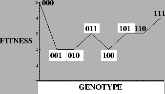
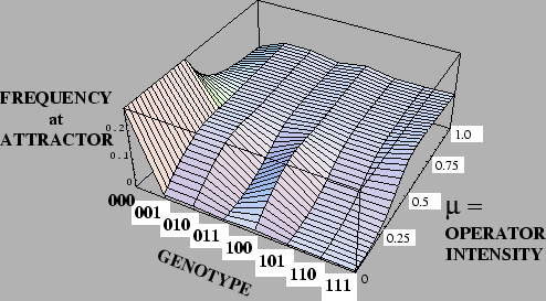
There is only one attractor at each value  , but an `error catastrophe' is evident for
 .
.
Finite Populations
- So why do evolutionary algorithms with ergodic mutation seem to get trapped on `local fitness peaks'? e.g. Kauffman's NK Landscapes?
- Answer: finite population size causing genetic drift: small random samples have stochastic variation, and types with few copies tend to go extinct rather than grow exponentially.
Fisher's Result on the Survival of a Fitter Mutant
- Fisher, R. A. 1930. The genetical theory of natural selection. Oxford: Clarendon Press.
Result 2
Suppose that,
- in a large population of individuals that produce an average of 1 offspring each,
- a new mutant appears that produces a average of 1 + s offspring,
- with variance
 ,
and where s is small.
,
and where s is small.
The probability that the fitter mutant will not eventually go extinct is

.
The Wright-Fisher Model of Finite Populations
- Wright, S. 1931. Evolution in Mendelian populations. Genetics 16:97-159.
- Fisher, R. A. 1930. The genetical theory of natural selection. Oxford: Clarendon Press.
How can an evolutionary algorithm with finite population size be modelled? Wright and Fisher had the same idea for modelling for finite populations.
Wright-Fisher Model
Suppose that each individual of the next generation be created by independent application of selection and genetic operators to the population.
Let:
- N
- be the population size;
-

- be a vector of the number of individuals of each type i in the population;
-

- be the probability a new individual of type i is generated by selection and genetic operators acting on the population
 .
.
Then the chance
 that there are
  individuals of type i in next generation is:
The Wright-Fisher model forms a Markov chain. Wright and Fisher analyzed many of the properties of this Markov system, including probabilities of fixation, time to fixation, and stationary distributions of allele frequencies.
The theory of Wright and Fisher is known in the Evolutionary Computation community as the `Nix and Vose model':
- A. E. Nix and M. D. Vose, 1991, Modeling genetic algorithms with Markov chains, Annals of Mathematics and Artificial Intelligence 5: 79-88.
Karlin's Theorem on
Genetic Operator Intensity
- Karlin, Samuel. 1982. Classifications of selection-migration structures and conditions for a protected polymorphism. In Hecht, M. K. and B. Wallace and G. T. Prance, Evolutionary Biology 14: 61--204.
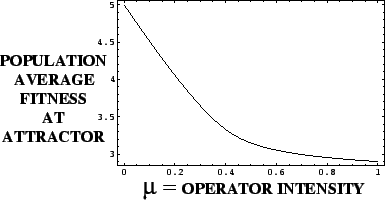
Result 3
Consider an evolutionary algorithm consisting of
- constant selection, and
- asexual genetic operators.
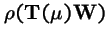
The mean fitness of the population at an attractor is a decreasing function of the probability of the genetic operator acting.
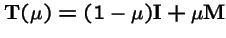
How is this obtained? Let the asexual genetic operator be represented by the Markov matrix , and let is the probability of applying the operator. Then the transmission matrix for the algorithm is:
and the recursion is:
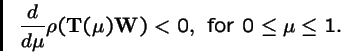
Karlin's Theorem, continued.
Samuel Karlin developed a theorem to determine when alleles introduced into a multi-deme population would increase in number.
Theorem 3 (Karlin, 1982)
Let
,
where
is an irreducible Markov matrix, and let

be a strictly positive diagonal matrix. Then the spectral radius
is strictly decreasing in
:
For the global attractor,
 , which is the leading eigenvector of
 , we have:
Hence the mean fitness of the global attractor,
is a decreasing function of the operator probability .
Karlin's Theorem illustrated with the
Deceptive Function
=
Tensor (Kronecker) Products
- Roux, C. Z. 1974. Hardy-Weinberg equilibria in random mating populations. Theoretical Population Biology 5: 393-416.
- Feldman, M. W. and J. Krakauer. 1976. Genetic modification and modifier polymorphisms. pp. 547-583 in Population Genetics and Ecology, ed. S. Karlin and E. Nevo. Academic Press, New York.
- Karlin, S. and U. Liberman. 1978. The two-locus multi-allele additive viability model. J. Mathematical Biology 5: 201-211.
Useful for:
- Multiple Loci
- Sexual Reproduction
- Compound types: genotype
phenotype
deme
- Compound operators: mutation
recombination
migration
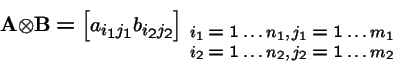
Tensor Products, continued
Let
and
Then the tensor product is:
In general,
Tensor Products for Compound States
Frequency Vector of Multiple Loci in Linkage Equilibrium, i.e. no allele associations between loci:
Frequency Vector of Genotypes Randomly Spread over Multiple Demes
where  is the vector of genotype frequencies and
is the vector of deme sizes (as fractions of the whole meta-population).
is the vector of genotype frequencies and
is the vector of deme sizes (as fractions of the whole meta-population).
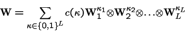
Tensor Products for Compound Operators
When multiple independent operators are acting on the types in the population, the compound operator can be represented by tensor products.
Mutation at Multiple Loci
Suppose locus k mutates with transition probabilities
Then the mutation operator acting on the entire genotype of L loci is:
Mutation + Recombination
When both recombination and mutation act independently on the genotype, the transmission function can be represented as (R=recombination, M=mutation, D=migration):
Mutation + Recombination + Migration
Generalized Nonepistatic Fitnesses (Karlin and Liberman 1979)
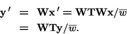
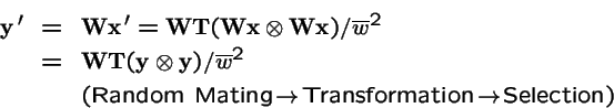
Selection and Transformation Commute:
Does the order
 vs.
vs.
 produce different evolutionary outcomes?
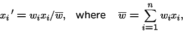
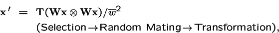
Assume frequency-independent selection:
Asexual:
Clearly,
 . However, make a change of variables: let
 , and
, and
 . Then:
So the operators
and
 produce the same trajectories with mapping between variables
.
produce the same trajectories with mapping between variables
.
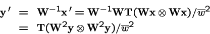
Sexual:
Again let
, and
.
Selection on both Parents and Offspring:
What is the effect of applying selection to the choice of parents, and then applying selection again to the offspring?
Now, make a change of variables: let
 , and
, and
 .
.
Hence
is equivalent to:
Gieringer's Representation of `all possible'
Crossover operators
- Geiringer, H. 1944. On the probability theory of linkage in Mendelian heredity. Ann. Math. Statist. 15: 25-57.
- Karlin, Sam and Uri Liberman. 1978. Classification and comparisons of multilocus recombination distributions. Proc. Natl. Acad. Sci. 75: 6332-6336.
Geiringer (1944) developed a way to represent all possible recombination operators acting on two parents. This includes single point, multiple point, and uniform crossover. She considered which genes get transmitted together into an offspring.
Gieringer, continued
- All the genes transmitted from one parent can be marked with a 0, and
- all the genes transmitted from the other parent can be marked with a 1.
- Hence a particular recombinant offspring can be represented as a binary string, e.g.
(0,1,1,0,1,1,0,0,0).
- Hence, the recombination operation corresponds to a mask
- There are
 possible such recombination operations.
- What defines a crossover operator is the probability of performing a particular recombination operation.
- Thus, a crossover operator can be defined as a probability distribution over the set of masks:
- Since every recombination event can produce an offspring with the genes from the reversed parents, we have the symmetry constraint that:
Representing the Mult-locus, Multi-Allele Model with Nonepistatic Selection and Arbitrary Crossover
- Karlin, Sam and Uri Liberman. 1979. Central equilibria in multilocus systems. I. Generalized nonepistatic selection regimes. Genetics 91: 777-798.
where each
![${\bf W}={\left[ \stackrel{}{w_{ij}}\right]}$](img99.gif) is a diploid fitness matrix.
is a diploid fitness matrix.
- Note: Haploidy is the special case where:
- Analytical solutions for the existence and stability of polymorphisms have been found for the general non-epistatic model.
- Generalized non-epistasis is a highly non-generic space of fitness functions.
- Trajectories and equilibria of the general epistatic model are unsolved in closed form.
Takeover Times
- Goldberg, D. and Deb. 1991. A comparative analysis of selection schemes used in genetic algorithms. In G. Rawlins, editor, Foundations of Genetic Algorithms, pages 69-93. Morgan Kaufmann, San Mateo, CA.
Goldberg and Deb use a `pseudo finite population' analysis:
- Let i be the fittest type;
- Calculate, in terms of n, the time for an infinite population to go from xi = 1/n to
xi = 1-1/n under selection alone.
- Problem: method does not take into account genetic drift in finite populations.
`Takeover Times' known in Population Genetics as Fixation Times
Keywords:
- Fixation:
- When only one variant remains in the populaton.
- Polymorphism:
- When more than one variant exists in the populaton.
- Fixation Time:
- Time until the population goes from polymorphism to fixation.
- Conditional Fixation Time:
- Time until fixation, given that the population fixes on specific genotype.
- Takeover Time:
- Time until the fittest type goes to fixation, given that the population fixes on it.
Literature on Fixation Times
- Fisher, R. A. 1930. The genetical theory of natural selection.
Oxford: Clarendon Press.
- Wright, S. 1931. Evolution in Mendelian populations. Genetics 16:97-159.
- Kimura, M. and T. Ohta. 1969. The average number of generations until fixation of a mutant gene in a finite population. Genetics 61: 763-771.
- Carr, R. N., and R. F. Nassar. 1970. Effects of selection and drift on the dynamics of finite populations. II. Expected time to fixation or loss of an allele. Biometrics 26: 221-227.
- Ohta, T., and M. Kimura. 1972. Fixation time of overdominant alleles influenced by random fluctuation of selection intensity. Genetical Research 20: 1-7.
- Nei, M., and A. K. Roychoudhury. 1973. Probability of fixation and mean fixation time of an overdominant mutation. Genetics 74: 371-380.
- Nassar, R. F., and R. D. Cook. 1974.
Ultimate probability of fixation and time to fixation or loss of a gene under a variable fitness model. Theoretical and Applied Genetics 44: 247-254.
- Ewens, W. J.. 1979. Mathematical Population Genetics. Springer-Verlag, Berlin.
Conditional Fixation Time
of a Fitter Allele
- Kimura, M. and T. Ohta. 1969. The average number of generations until fixation of a mutant gene in a finite population. Genetics 61: 763-771.
About this document ...
Lee Altenberg
2000-08-29
![\begin{displaymath}{\bf A}= {\left[ \stackrel{}{
\begin{array}{ccc}
a_{11} & a_{12} & a_{13}\\
a_{21} & a_{22} & a_{23}
\end{array}}\right]},
\end{displaymath}](img65.gif)
![\begin{displaymath}{\bf B}= {\left[ \stackrel{}{
\begin{array}{ccc}
b_{11} & b_{...
...\\
b_{31} & b_{32} \\
b_{41} & b_{42}
\end{array}}\right]},
\end{displaymath}](img66.gif)
![\begin{eqnarray*}{\bf A}\otimes {\bf B}&=& {\left[ \stackrel{}{
\begin{array}{cc...
...2} b_{42} & a_{23} b_{41} & a_{23} b_{42}
\end{array}}\right]}.
\end{eqnarray*}](img67.gif)
![\begin{displaymath}{\cal R}: \{0, 1\}^L \mapsto [0, 1]: \; \sum_{{\bf c}\in\{0, 1\}^L} {\cal R}({\bf c}) = 1
\end{displaymath}](img96.gif)

![\begin{displaymath}{\bf W}= {\bf w}{\bf w}^{{\rm T}}, \;\;{\bf w}= {\left[ \stackrel{}{\begin{array}{c}w_1\\ \vdots\\ w_L\end{array}}\right]}.
\end{displaymath}](img100.gif)